How to use Conditional Formatting in Excel to Color-Code Specific Cells
Sign up to receive The Snapshot, a free special dispatch from Laptop Mag, in your inbox.
You are now subscribed
Your newsletter sign-up was successful
Selecting individual cells -- even by Ctrl + clicking to choose multiple cells -- is a timesink. In Excel, it’s best to make use of Conditional Formatting for otherwise tedious tasks, such as this one.
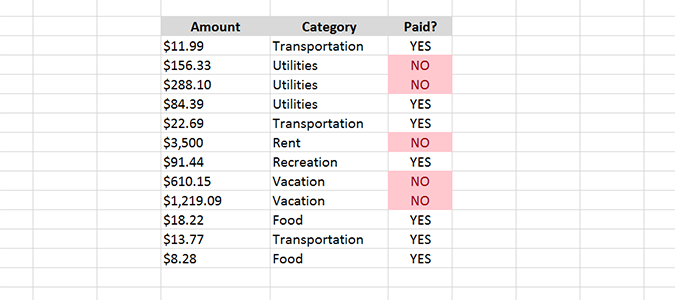
In fact, it’s an easy argument to make that aside from Pivot Tables, Conditional Formatting is Excel’s most useful feature. Conditional Formatting essentially allows you to set specific rules in an if/then sort of language. Using our spreadsheet below, we can create easy rules to color code bills that have yet to be paid. Or, we could apply Conditional Formatting to bills we’ve paid, while adding a second condition to color code everything in the “utilities” category.
- Learn how to Remove Duplicate Entries in Excel
- Learn how to create a Pivot Table based on Multiple Tables in Excel 2013
- Here's how to Add a Drop-Down List in Excel
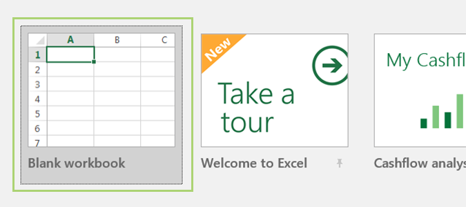
1. Open a workbook in Excel. For the sake of this tutorial, I’m going to fill it with dummy data. You can do the same, or work from an existing workbook; just be sure to save it first.
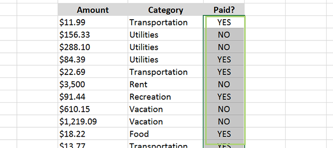
Article continues below2. Select the data to be formatted. In this case, we’re going to choose everything in Column G, the “Paid?” category.
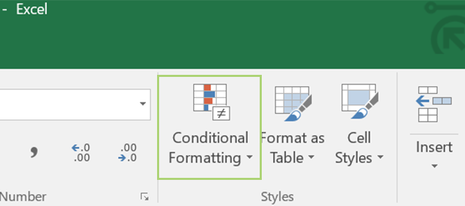
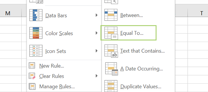
3. Choose Conditional Formatting from the ribbon.
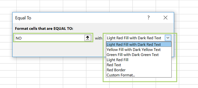
5. We’re going to color-code bills that we haven’t paid. To do that, add “NO” to the Format cells that are EQUAL TO box, and then select a color option from the dropdown menu. Or, you can create your own using Custom Format…
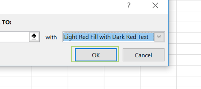
6. Press OK.
Sign up to receive The Snapshot, a free special dispatch from Laptop Mag, in your inbox.
- Learn how to Remove Duplicate Entries in Excel
- Learn how to create a Pivot Table based on Multiple Tables in Excel 2013
- See how to use Conditional Formatting in Excel to Color-Code Specific Cells
Bryan covers everything you need to know about Windows, social media, and the internet at large for Laptop Mag. Thanks to his extensive knowledge of operating systems and some of the most popular software out there, Bryan has written hundreds of helpful guides, including tips related to Windows 11 drivers, upgrading to a newer version of the OS, editing in Microsoft Photos, or rearranging pages in Google Docs.
