How to use VLOOKUP in Excel
The one Excel trick you need to know is how to use VLOOKUP
Sign up to receive The Snapshot, a free special dispatch from Laptop Mag, in your inbox.
You are now subscribed
Your newsletter sign-up was successful
Microsoft Excel 2016 boasts a huge number of handy functions and utilities, many of which go untouched by the average user. If you find yourself repeatedly consulting the same table to find data, however, have a gander at VLOOKUP. Short for "vertical lookup," VLOOKUP takes advantage of vertically-aligned tables to quickly locate data associated with a given value.
Note: though this tutorial was written for Microsoft Excel 2013, it works the same way in the latest version of Excel.
- Here's how to freeze rows in Excel and how to recover a deleted or unsaved Excel file
- How to Create a Sortable Column in an Excel Workbook
- Check out our Excel tips roundup
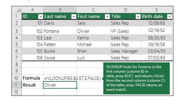
If you know the name of a product, for instance, and you want to quickly determine its price, simply enter the product name into Excel and VLOOKUP will find the price for you. To the novice Excel user, setting up VLOOKUP can look like an intimidating process — but it needn't be. Just follow our step-by-step tutorial on how to use VLOOKUP in Excel today.
How to use VLOOKUP in Excel
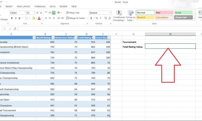
1. Click the cell where you want the VLOOKUP formula to be calculated.
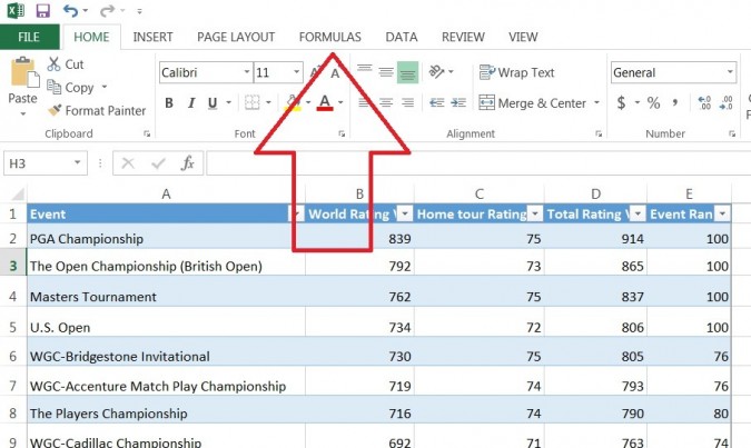
2. Click Formulas at the top of the screen.
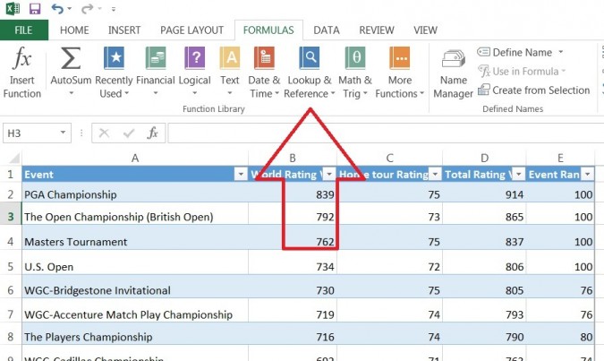
3. Click Lookup & Reference on the Ribbon.
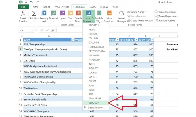
4. Click VLOOKUP at the bottom of the drop-down menu.
Sign up to receive The Snapshot, a free special dispatch from Laptop Mag, in your inbox.
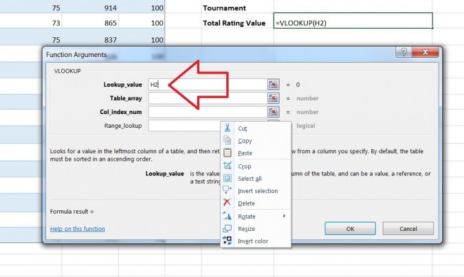
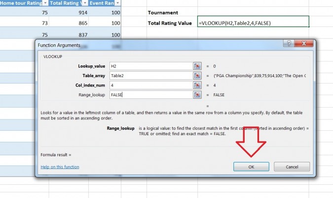
5. Specify the cell in which you will enter the value whose data you're looking for. In this case, our lookup value is H2, since this is where we will input the name of a tournament such as "PGA Championship," so we input "H2" in the lookup_value box of the popup window. Once we've set up VLOOKUP properly, Excel will return the tournament's Total Rating Value in cell H3 when we type the tournament name in cell H2.
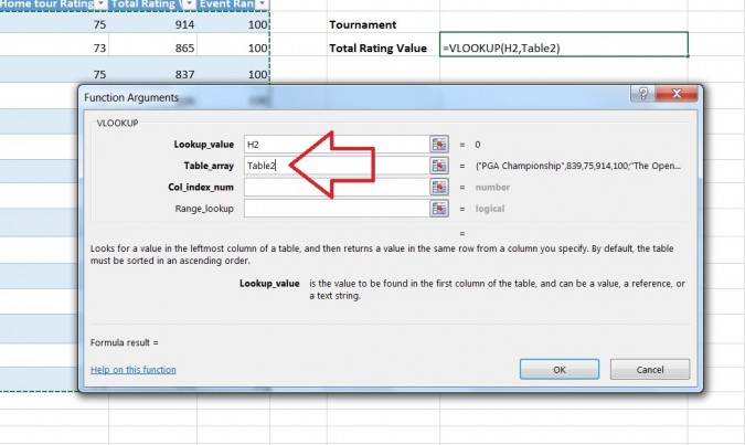
6. Specify the data that you want VLOOKUP to use for its search in the table_array box. In this case, we've selected the entire table (excluding the headers).
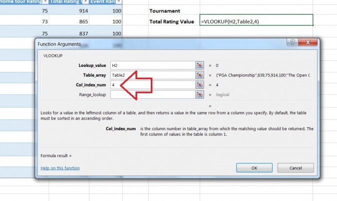
7. Specify the column number which VLOOKUP will use to find the relevant data in the col_index_num box. Somewhat confusingly, VLOOKUP requires you to use the numerical value of the column rather than its letter value. In this case, we want VLOOKUP to use the Total Rating Value column — column D — so we enter the number 4.
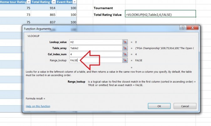
8. Specify whether you need an exact match by entering either FALSE (exact match) or TRUE (approximate match) in the range_lookup box. In this case, we want an exact match so we enter FALSE.
9. Click OK at the bottom of the popup window.
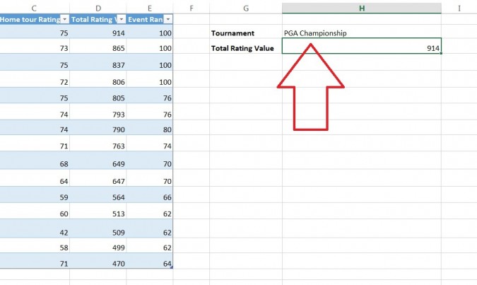
10. Enter the value whose data you're searching for. In our example, we want to find the Total Value Rating of the PGA Championship, so we type "PGA Championship" into cell H2 and VLOOKUP automatically produces the Total Value Rating (in this case, 914) in cell H3.
Using VLOOKUP, you can not only search for individual values, but also combine two worksheets into one. For example, if you have one worksheet with names and phone numbers and another sheet with names and email addresses, you can put the email addresses next to the names and phone numbers by using VLOOKUP.
More Microsoft Excel tips and tricks
There are a number of neat tips that'll help you out when you're managing your Excel spreadsheets. For example, when you protect a sheet or workbook, all of the cells will be locked, but you can also lock cells individually by right-clicking and selecting "Format Cells." And if you need to, you can also freeze rows and columns by selecting "Freeze Panes" in the View tab.
But not everyone is a fan of Excel, so if you need to convert Excel spreadsheets to Google Sheets, we have a guide for that, as well as a guide on how to open Google Sheets in Excel.
For business users, we also have 10 Excel business tips that can help you keep your job, including guides on how to remove duplicate data, recover lost Excel files, use pivot tables to summarize data, and more.
We even have guides on how to use conditional formatting in Excel to color-code specific cells and how to add comments to your formulas in Microsoft Excel.
- How to upgrade to Office 2016
David was a writer at Laptop Mag. His coverage spanned how-to guides, reviews, and product rankings. He reviewed Asus, Lenovo, and Gigabyte laptops; guided readers on how to do various things in Excel, and even how to force quit an app in macOS. Outside of Laptop Mag, his work has appeared on sites such as Tom's Guide and TechRadar.
