How to Add Conditional Formatting in Excel 2013
Sign up to receive The Snapshot, a free special dispatch from Laptop Mag, in your inbox.
You are now subscribed
Your newsletter sign-up was successful
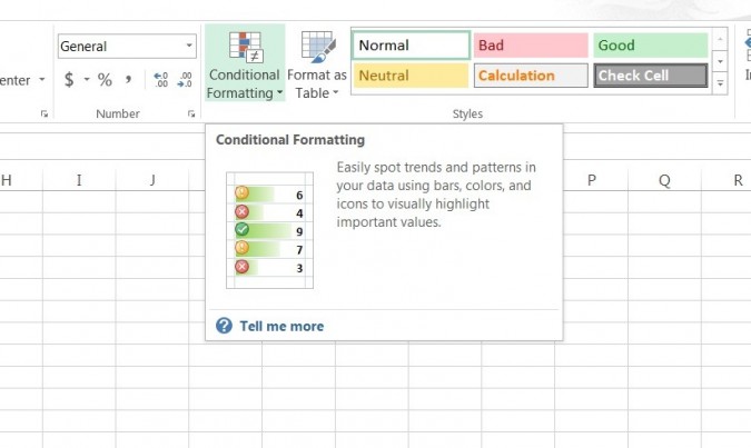
Microsoft Excel 2013 introduces a new feature that lets you differentiate data at a glance: Conditional formatting. This handy tool will apply colors to a cell's font and background depending on the conditions you've set -- if you want to highlight any cell that features a specific name or date, for instance, or differentiate high, medium and low numerical values. Follow these directions to set up your own conditional formatting in a few simple steps.
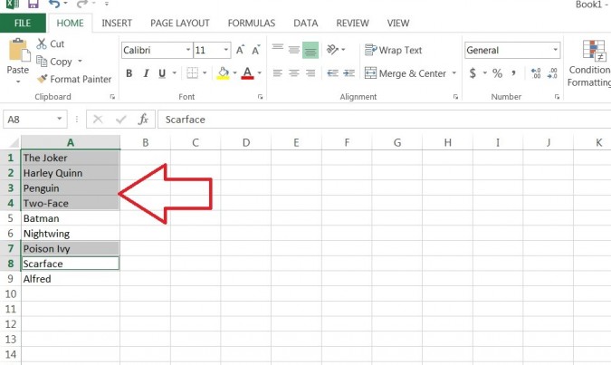
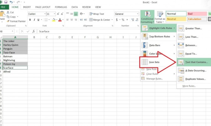
1. Select the cells you want to format.
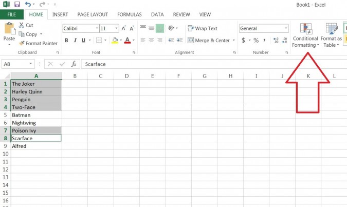
2. Click "Conditional Formatting" on the Ribbon.
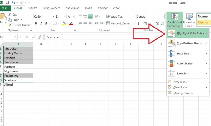
3. Hover over "Highlight Cells Rules" in the drop-down menu.
4. Click on "Text that Contains" in the drop-down menu.
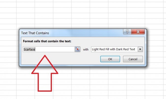
5. Select the text you want formatted in the "Text that Contains" popup window.
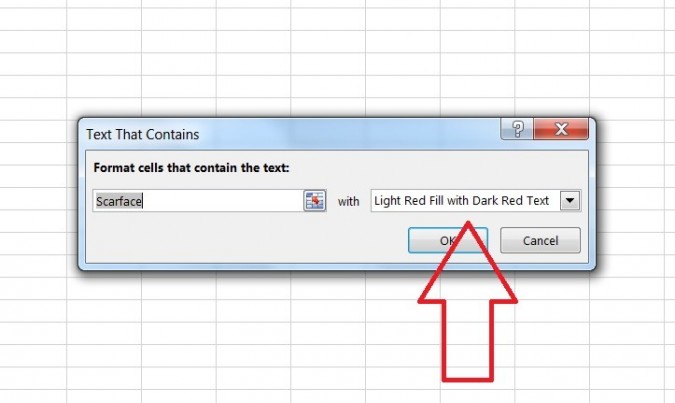
6. Choose the format in the "Text that Contains" popup window.
Sign up to receive The Snapshot, a free special dispatch from Laptop Mag, in your inbox.
- 15 Pieces of Software to Install on Your New PC
- Best Laptops 2013
- 8 Worst Windows 8 Annoyances and How to Fix Them
David was a writer at Laptop Mag. His coverage spanned how-to guides, reviews, and product rankings. He reviewed Asus, Lenovo, and Gigabyte laptops; guided readers on how to do various things in Excel, and even how to force quit an app in macOS. Outside of Laptop Mag, his work has appeared on sites such as Tom's Guide and TechRadar.
