Working on a Microsoft Excel spreadsheet can be pretty labor intensive. But learning how to transpose columns and rows using Paste Special in Excel can make life easier.
Traditionally, you make various rows and columns, then enter all of the information, but it can be a lot to keep track of. After incorrectly entering data, one of the most common mistakes is transposing columns and rows. You know, when you accidentally put the names at the top of each column instead of the dates, or vice-versa. The same goes for rows -- instead of adding the data you wanted in the column, you’re now stuck with a row-formatted data entry.
- Check how to Use VLOOKUP in Excel and Back Up Files Automatically in Excel
- How to Remove Duplicate Data in Excel and Create a Waterfall Chart in Excel
- This is how to protect cells, columns, and rows from accidental editing in Excel
With Excel, you might think the only option is to copy/paste the entries into the correct place, or start over. But, this would be wrong. There’s a really easy fix in the Paste Special menu that allows you to reverse your mistakes and columns to rows without starting over. You're going to transpose everything. Transposing excel columns to rows basically means that you're switching or rotating information from one row or column to another.
Transposing rows to columns in Excel is pretty easy. Even better, Google Sheets, OpenOffice and most spreadsheet applications have near identical functionality. Here's how to transpose columns to rows and vice-versa in Microsoft Excel.
How to transpose columns and rows using Paste Special in Excel
1. Open Excel and choose Blank workbook.

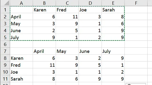
2. Enter the data you’d like to shift around from a column to a row (or vice versa).

3. Copy the entire data set by selecting each area, right-clicking, and selecting Copy.

4. Click on a new location in the sheet to add your transposed data.

5. Right click and choose Paste Special. Alternatively, you can use the keyboard shortcut Ctrl + Alt + V.

6. At the bottom of the Paste Special box, check the Transpose option.

7. Press OK to transpose the columns and rows.