How to lock cells in Excel
This is how to protect cells in Excel
Sign up to receive The Snapshot, a free special dispatch from Laptop Mag, in your inbox.
You are now subscribed
Your newsletter sign-up was successful
You've worked hard on your spreadsheet and now you want to make sure anyone you share it with doesn't inadvertently change cells, so you need to know how to lock cells in Excel.
Thankfully, Microsoft Excel 2016 and earlier versions lets you lock cells or protect cells to keep them from being modified in Windows 10. You can lock all the cells in a worksheet or specific cells, allowing some parts of the spreadsheet to be changed. Here's how to lock cells in Excel.
Editor's Note: This tutorial was written for Excel 2016, but still applies to modern versions of Excel.
How to lock all the cells in an Excel worksheet
By default, when you protect cells in a sheet or workbook, all of the cells will be locked. This means they can't be reformatted or deleted, and the content in them can't be edited. By default, the locked cells can be selected, but you can change that in the protection options.
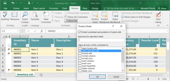
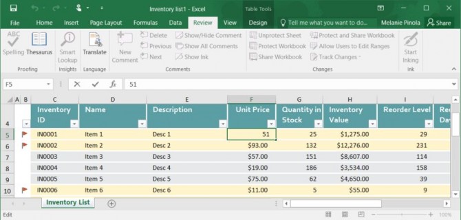
1. Navigate to the Review tab.
2. Click Protect Sheet. In the Protect Sheet window, enter a password that's required to unprotect the sheet (optional) and any of the actions you want to allow users.
3. Click OK to protect the sheet.
Sign up to receive The Snapshot, a free special dispatch from Laptop Mag, in your inbox.
When you or anyone else tries to edit any of the locked cells, this message will come up:
The cells can only be unlocked when the sheet is unprotected (by going to the Review tab again, choosing "Unprotect Sheet," and entering the password, if required).
How to Lock Specific Cells in an Excel Worksheet
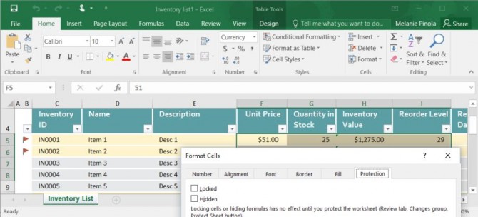
There might be times when you want to lock certain cells from being changed but still allow users to adjust other cells in a worksheet. In our example, in an inventory list you might allow unit prices and stock quantities to be updated, but not the item IDs, names, or descriptions. As mentioned above, all cells are locked by default when you protect the sheet. However, you can specify whether a certain cell should be locked or unlocked in the cell's format properties.
1. Select all the cells you don't want to be locked. These will be the specific cells that can be edited even after the sheet is protected.
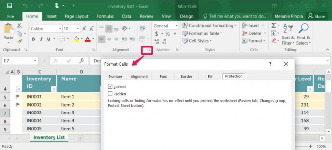
2. Right-click on your selection, select Format Cells, and click on the Protection tab. (Alternatively, under the Home tab, click on the expansion icon next to Alignment, and in the Format Cells window go to the Protection tab.)
3. Uncheck "Locked" (which is checked by default) and click OK.
4. Go to Review > Protect Sheet and hit OK to protect the sheet. Any cells you didn't unlock under the Format Cells option (step 3 above) will be locked, while the unlocked cells will be editable:
Note that locking (or unlocking) specific cells won't take effect until you do step 4, protecting the sheet.
Protip: If you want to quickly lock or unlock cells that aren't next to each other, you can use a keyboard shortcut. After selecting a certain cell or group of cells, use the Format Cells dialog as above to lock or unlock it. Then select your next cell(s) and hit F4 to repeat your last action.
More Microsoft Excel tips and tricks
There are a number of neat tips that'll help you out when you're managing your Excel spreadsheets. For example, we have a guide on how to use VLOOKUP in Excel, which you can use to to quickly find data associated with a value the user enters. And if you need to, you can also freeze rows and columns by selecting "Freeze Panes" in the View tab. If you need to organize your data, check out how to create sortable columns in Excel.
But, not everyone is a fan of Excel, so if you need to convert Excel Spreadsheets to Google Sheets, we have a guide for that, as well as a guide on how to open Google Sheets in Excel.
If you're a business users, we also have 10 Excel business tips that you can use to help you keep your job, which include guides on how to remove duplicate data, recover lost Excel files, use pivot tables to summarize data and more.
We even have guides on how to use conditional formatting in Excel to color-code specific cells and how to add comments to your formulas in Microsoft Excel.
Melanie was a writer at Laptop Mag. She wrote dozens of helpful how-to guides, covering both the software and the hardware side of things. Her work included topics like SSDs, RAM, Apple, Excel, OneDrive, and detailed guides for Windows users. Outside of all her useful advice, Melanie also penned a few reviews for Laptop Mag, including Android emulators that help you run apps on your PC.
