How to Create a Pivot Table Based on Multiple Tables in Excel 2013
Sign up to receive The Snapshot, a free special dispatch from Laptop Mag, in your inbox.
You are now subscribed
Your newsletter sign-up was successful
Up until recently, if you had data spread across several tables in Microsoft Excel that you wanted to consolidate in a single pivot table, you would have faced a headache-inducing process of manual formatting and data preparation. The most recent version of the software, Excel 2013, fixes this problem by allowing you to create a pivot table from multiple tables automatically -- no manual formatting required. Just follow these steps to get started.
- Learn how to Remove Duplicate Entries and how to add decimal points in Excel
- Here's how to Add a Drop-Down List in Excel
- See how to use Conditional Formatting in Excel to Color-Code Specific Cells
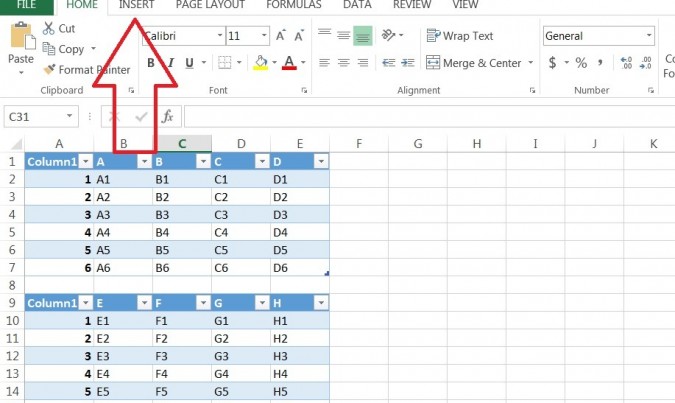
1. Click "Insert" at the top of the screen.
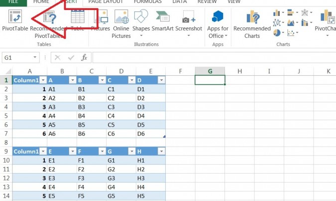
2. Click the "PivotTable" button on the Ribbon.
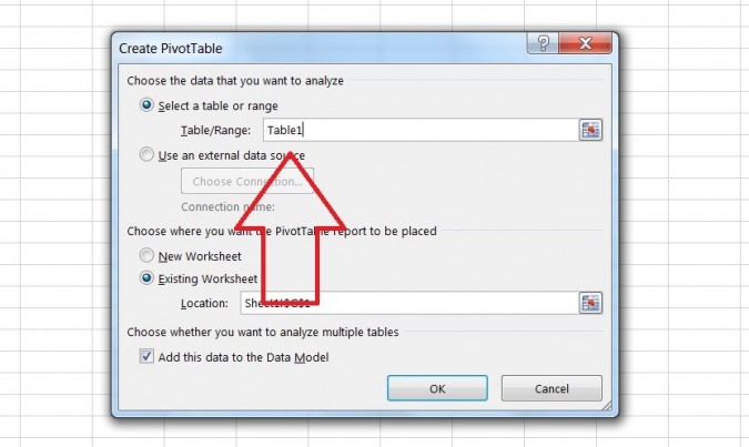
Article continues below3. Select the first table you want to add to the pivot table.
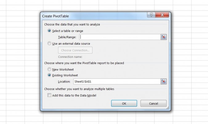
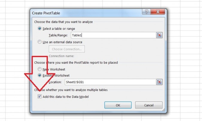
4. Check the box labeled "Add this data to the Data Model" and press OK.
5. Click "All" in the PivotTable Fields window to view all of the tables. Excel automatically detects multiple tables, so you won't need to repeat these steps for each additional table.
6. Check the boxes of the cells you wish to include in the pivot table.
Sign up to receive The Snapshot, a free special dispatch from Laptop Mag, in your inbox.
- 15 PC-Cleaning Tools to Speed Your Computer
- 8 Essential Tips for Your New Windows 8 PC
- 8 Laptop Buying Tips for Students
David was a writer at Laptop Mag. His coverage spanned how-to guides, reviews, and product rankings. He reviewed Asus, Lenovo, and Gigabyte laptops; guided readers on how to do various things in Excel, and even how to force quit an app in macOS. Outside of Laptop Mag, his work has appeared on sites such as Tom's Guide and TechRadar.
