When you ask people which Google Sheets functions they are familiar with, the most common answers you will get are SUM and IF. But what if I tell you that Google Sheets has a function that combines both? The SUMIF function will become one of your favorites after we delve into how it can streamline your workflow.
SUMIF allows you to combine values that satisfy the criteria you set. Based on this, you can already guess that the SUMIF function requires two parameters: the range of numbers you want to add together and the criteria that will determine which of these numbers to include.
By using the SUMIF function, you can save plenty of time from having to sort and filter your data. You are also more assured of your data’s accuracy, as the combination is conducted without manual intervention. Now that you are familiar with this function, here are the steps on how to use it.
How to use the SUMIF Function on Google Sheets
1. Open your spreadsheet and click on the cell where you want the output to appear.

2. You have two options to initiate the SUMIF function. While on your selected cell, you can go to Insert > Function > Math > SUMIF on your main header toolbar. You can also type =SUMIF( on your cell.

3. After initiating the function, you need to enter the first parameter range by highlighting your array of data.

4. Next, type a comma (,) and input your criterion.

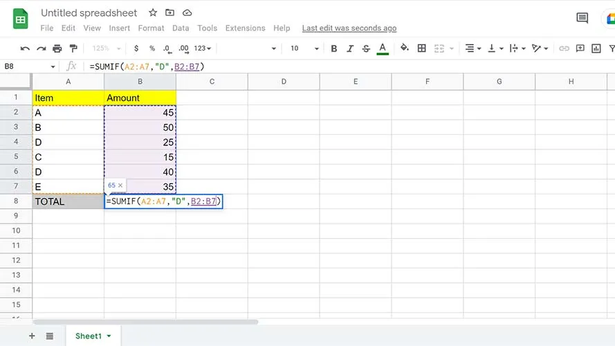
5. A third optional parameter is the sum_range. You only need to use the sum-range parameter if your values are different from your range. Using sum_range, Sheets compares your criterion to your range, then adds the values on the same row of range items that match your criteria.

6. Lastly, press Enter on your keyboard. Your output will appear in the cell.